
In this case, I want the work requests with a status of "Approved" to have a yellow background and those that have a status of "Clarification" required to have an orange background. I'd like the "Pending" and "Modified" requests to also have an orange background, but a different shade of orange. Since it doesn't matter to me if they share the same background color, I can use an "or" condition when creating the conditional formatting.
I can create the conditional formatting for a particular cell, e.g., B3, by clicking on Format then selecting Conditional Formatting and then specifying the following conditions using the Add button to add additional conditions and clicking on the Format button to select the colors I want for each condition.
| Condition 1 | ||
| Cell Value Is | equal to | ="Approved" |
| Condition 2 | ||
| Cell Value Is | equal to | ="Clarification Required" |
| Condition 3 | ||
| Formula Is | =OR(B3="Pending",B3="Modified") | |
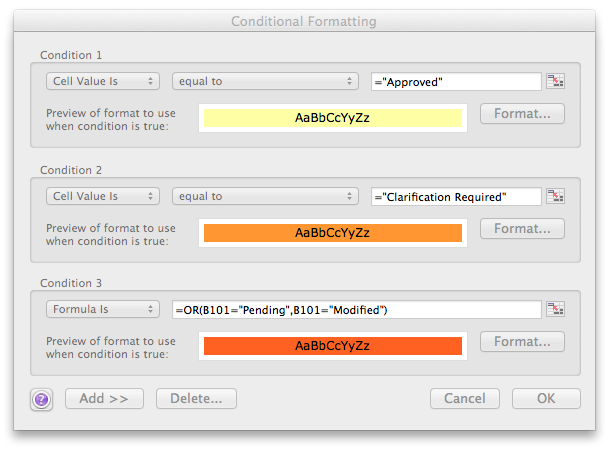
For the last condition, I use "Formula Is" rather than "Cell Value Is",
so that I can use the Or operator which won't work if I pick
"Cell Value Is". The following steps will then allow me to apply
the desired conditional formatting to all cells in the relevant
column.
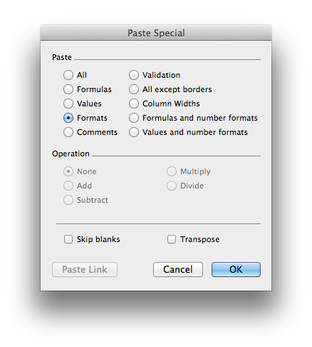
When the conditional formatting is copied, the relevant cell number will be adjusted for each cell. I.e., B3, which was in the formula I copied, will be replaced with the appropriate cell reference.
With the conditional formatting applied, when I scroll through the list of hundreds of work requests, I can easily identify the ones needing attention.
![]()
Created: Thursday February 26, 2015