
=(TODAY()-F16)<7 for
conditional formatting for cell F16 (row 16 column F), if that cell holds an
approval date. I.e., if today is Tuesday, December 8, 2009 and
I only want the cell color to change if a request was approved since the
prior Tuesday, December 1, 2009, I can take the following steps in
Excel (note these steps were written for Excel 2007, but should work for
versions of Excel since Excel 95, which supported conditional formatting):
=(TODAY()-F16)<7 in the formula field.

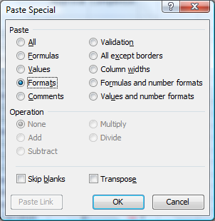
I want the conditional formatting to apply to all cells holding approval dates in a spreadsheet, not just one particular cell. To apply the same conditional formatting to other cells in column F holding approval dates, I would select the cell holding the conditional formatting by clicking on it, then select Edit and Copy. I can then highlight other cells and apply the same conditional formatting to them. E.g., I could highlight the column for all rows except for the column heading. Once I've highlighted the cells to which the conditional formatting should apply, I can click on Edit then select Paste Special. I can then click on the Formats radio button to select Formats, then click on OK.

References: