
offset function that allows
you to calculate a value based on the contents of a cell that is a specified
distance in rows and columns from a particular cell. The syntax for calc is
as follows:
OFFSET
Returns the value of a cell offset by a certain number of rows and columns from a given reference point.
Syntax
OFFSET(Reference; Rows; Columns; Height; Width)
Reference is the reference from which the function searches for the new reference.
Rows is the number of rows by which the reference was corrected up (negative value) or down.
Columns (optional) is the number of columns by which the reference was corrected to the left (negative value) or to the right.
Height (optional) is the vertical height for an area that starts at the new reference position.
Width (optional) is the horizontal width for an area that starts at the new reference position.
Arguments Rows and Columns must not lead to zero or negative start row or column.
Arguments Height and Width must not lead to zero or negative count of rows or columns.
In the OpenOffice Calc functions, parameters marked as "optional" can be left out only when no parameter follows. For example, in a function with four parameters, where the last two parameters are marked as "optional", you can leave out parameter 4 or parameters 3 and 4, but you cannot leave out parameter 3 alone.Example
=OFFSET(A1;2;2) returns the value in cell C3 (A1 moved by two rows and two columns down). If C3 contains the value 100 this function returns the value 100.
=OFFSET(B2:C3;1;1) returns a reference to B2:C3 moved down by 1 row and one column to the right (C3:D4).
=OFFSET(B2:C3;-1;-1) returns a reference to B2:C3 moved up by 1 row and one column to the left (A1:B2).
=OFFSET(B2:C3;0;0;3;4) returns a reference to B2:C3 resized to 3 rows and 4 columns (B2:E4).
=OFFSET(B2:C3;1;0;3;4) returns a reference to B2:C3 moved down by one row resized to 3 rows and 4 columns (B2:E4).
=SUM(OFFSET(A1;2;2;5;6)) determines the total of the area that starts in cell C3 and has a height of 5 rows and a width of 6 columns (area=C3:H7).
As another example, I have a Calc spreadsheet for tracking fund/stock performance in a 401(k) like plan. I want to track daily differences, i.e., the gain or loss from one day to the next, but also the overall gain or loss since I started tracking performance of the fund and also the overall increase or decrease in the per share price since I started tracking the performance. I have 7 columns in the spreadsheet. The first is the date, the second the number of shares, then the price per share for that day, and the amount of money for that day, i.e., shares times share price. For the next 3 columns I wanto to track how much the balance fluctuates from day to day (Daily $ Difference), the amount of increase or decrease in the overall balance from the day I first started tracking, which was March 13, 2015 (Overall $ Difference), and then also the amount the share price has increased or decreased since the day I started tracking, i.e., from March 13. The spreadsheet contains the information below:
| A | B | C | D | E | F | G | |
|---|---|---|---|---|---|---|---|
| 1 | Date | Shares | Share Price | Balance | Daily $ Difference | Overall $ Difference | Overall Share Price Difference |
| 2 | 03/13/15 | 2,146.7304 | $25.0525 | $53,780.96 | |||
| 3 | 03/14/15 | 2,146.7304 | $25.0525 | $53,780.96 | $0.00 | $0.00 | $0.00 |
| 4 | 03/15/15 | 2,146.7304 | $25.0525 | $53,780.96 | $0.00 | $0.00 | $0.00 |
| 5 | 03/16/15 | 2,146.7304 | $25.2853 | $54,280.72 | $499.76 | $499.76 | $0.23 |
| 5 | 03/17/15 | 2,146.7304 | $25.2683 | $54,244.23 | -$36.49 | $463.26 | $0.22 |
| 7 | 03/18/15 | 2,146.7304 | $25.9207 | $55,644.75 | $1,400.53 | $1,863.79 | $0.87 |
| 8 | 03/19/15 | 2,146.7304 | $25.5533 | $54,856.05 | -$788.71 | $1,075.08 | $0.50 |
| 9 | 03/20/15 | 2,146.7304 | $26.0621 | $55,948.30 | $1,092.26 | $2,167.34 | $1.01 |
| 10 | 03/21/15 | 2,146.7304 | $26.0621 | $55,948.30 | $0.00 | $2,167.34 | $1.01 |
| 11 | 03/22/15 | 2,146.7304 | $26.0621 | $55,948.30 | $0.00 | $2,167.34 | $1.01 |
| 12 | 03/23/15 | 2,146.7304 | $26.2510 | $56,353.82 | $405.52 | $2,572.86 | $1.20 |
| 13 | 03/24/15 | 2,162.4517 | $26.2562 | $56,777.76 | $423.94 | $2,996.80 | $1.20 |
| 14 | 03/25/15 | 2,162.4517 | $26.1116 | $56,465.07 | -$312.69 | $2,684.11 | $1.06 |
| 15 | 03/26/15 | 2,162.4517 | $25.8985 | $56,004.26 | -$460.82 | $2,223.29 | $0.85 |
| 16 | 03/27/15 | 2,166.1710 | $25.8811 | $56,062.89 | $58.63 | $2,281.92 | $0.83 |
| 17 | 03/28/15 | 2,166.1710 | $25.8811 | $56,062.89 | $0.00 | $2,281.92 | $0.83 |
| 18 | 03/29/15 | 2,166.1710 | $25.8811 | $56,062.89 | $0.00 | $2,281.92 | $0.83 |
| 19 | 03/30/15 | 2,166.1710 | $25.8994 | $56,102.53 | $39.64 | $2,321.57 | $0.85 |
| 20 | 03/31/15 | 2,166.1710 | $25.5993 | $55,452.46 | -$650.07 | $1,671.50 | $0.55 |
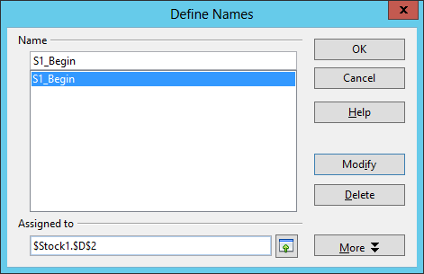
Since I may want to later insert data from days prior to March 13, rather
than reference cell D2 as the one to use for calculations for
the Overall $ Difference values, I defined a name to reference
that cell, instead of referencing it directly in formulas by clicking on
Insert, then Names, then Define. Since I had clicked
on the cell D2 in the sheet named Stock1 before selecting
Insert, $Stock1.$D$2 was already inserted for me in the
Assigned to field. I gave it the name S1_Begin.
Then in cell F3, I inserted the formula =D3-S1_Begin
to calculate the difference between D3 and D2,
since S1_Begin refers to the value in D2, for
the difference in dollars between the balance on March 14 and the balance on
March 13. I then copied the formula down to the last cell in the column,
so that cell F20 contained the formula =D20-S1_Begin.
Then, rather than create another defined name to calculate the share
price difference between a particular day and the price on the day I
first started tracking the share price, I inserted the formula
=C3-OFFSET(S1_Begin; 0; -1) in the cell G3. I then
copied that formula down to the last used cell in column G, so the formula
there is =C20-OFFSET(S1_Begin; 0; -1). That formula instructs
Calc to take the value of the current share price in cell D20
and then look at the value in the same row, row 20, indicated by the
zero after S1_Begin, i.e., the value in D2, but
the value in the column that is one column to the left of D2,
i.e., C2, which is indicated by the minus one which is then
subtracted from C20.
By using OFFSET in the formula, I don't have to create a second
defined name. Though, for this instance that wouldn't have been much additional
effort to create it and modify it if I later changed the start date for
calculations, since I have a number of sheets in this particular spreadsheet
it reduces the number of names I have to create and update overall to have
just one per sheet. I could also have made the first date, i.e., the contents
of cell A2 the value for S1_Begin and then used
OFFSET in column F calculations as well. E.g., if I had referenced
the first date, 03/31/15 in A2 for the defined name S1_Begin
, I could have put =C3-OFFSET(S1_Begin; 0; 2) for the
formula in cell G3. Then I would be referencing the column two
columns to the right of the referenced cell S1_Begin, since
the share price is two columns to the right of the date.
![]()
Created: Sunday April 12, 2015