Conditional Formatting in a Google Docs Spreadsheet

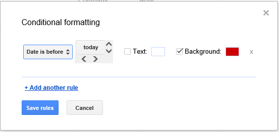
You can use conditional formatting in Google Docs spreadsheets to change the color of text in a cell or the background color of a cell just as you can in Microsoft Excel. E.g., if I had a cell that contained an expiration date and wanted the background color of the cell to be red if the date had been reached or had passed, I could click in the cell and take the following steps:

1. Click on Format.
2. Select Conditional formatting....
3. I could then select "Date is before" in the first field and "today" in the next field. I could then check "Background" and select the color red for the background color for the cell once the date in the cell has been passed.
4. Once you've set up the rule or rules for the cell or range of cells, clik on Save rules.

The cell will then have the normal color as long as the date stored in the cell is before today's date. Once the date in the cell matches today's date or is before the date of viewing, the cell background color will turn red.

Note: You can ensure that Google knows the cell contains a date by clicking on Format, selecting Number, and then More formats, which will allow you to pick a particular format you wish to use for dates, such as 2008-09-26, 9/26/08, etc.

[/network/web/services/google] permanent link

Kindle Fire Won't Power On

Yesterday, I found my Kindle Fire would not power on. I had used it a few hours earlier without seeing any message about the battery charge being low. But repeated attempts to turn it on by hitting the power button did no good. So I plugged it into a charger. Hours later when I attempted to power it on, I still was unable to do so. Following advice posted at My kindle won't turn on, I found that holding in the power button for 30 seconds then releasing the button and then tapping the power button again resulted in it powering on again. When it powered on, I saw the battery had a full charge.

[/ebook] permanent link