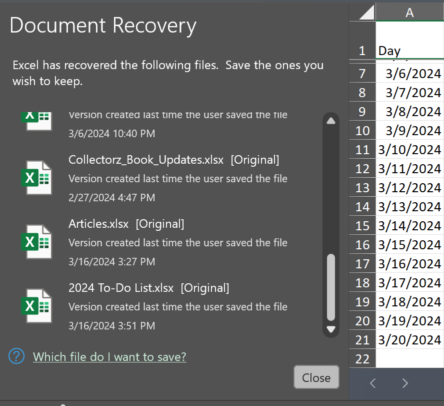
Microsft Excel can automatically save updates to spreadsheets. If Excel, or
the system, crashes, when you reopen Excel you will see a Document Recovery
pane on the left side of the Excel window with the message "Excel has
recovered the following files. Save the ones you wish to keep."
Some of the documents listed may have been saved by the user without any
subsequent changes being made and will have "Version created last time the
user saved the file" beneath the file name as shown above.
I inherited an Excel spreadsheet containing names and addresses for all the
members of an organization where all the letters for the names and addresses
were capitalized. I wanted to convert the names and addresses to "proper case"
where only the first letters of names, streets, and cities are capitalized
(in the
Python programming language proper case is known as "title case").
Fortunately, Excel provides a function, propercase, to perform that function.
To perform the conversion, I inserted a new column to the right of each of the
columns where all uppercase letters were used. The first column in the
Excel workbook contained the last names for the members. There was a header
titled "Last Name" in cell A1 with the first person's last name appearing in
cell A2, so in the newly inserted column, B, I put =proper(A2) in
cell B2. When I hit Enter, instead of AIKIN, JR in A2, I
then had Aikin, Jr in B2. I then clicked in cell B2 and dragged the
mouse pointer downwards to the last row containing a member's contact
information, which resulted in all the members last names being placed in
column B with the proper case, i.e., uppercase letters for the first letter of
the name and lowercase letters for the rest of the name. I couldn't just
delete column A then, which would cause a #REF! message to appear
in column B for every name, since I was using a formula that depended on
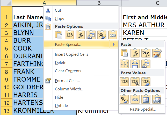
a value being in column A. So, instead, I copied all of column B by clicking
on the B at the top of the column to highlight all entries in
the column. I then used the Ctrl-C keys to copy all of the entries. I then
needed to paste the values in column B into column A, rather than pasting in
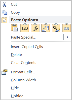
the formulas. You can do so, by right-clicking on the column designator
letter, i.e.the A for column A in this case, and then choosing
the appropriate paste option, To paste just the values and not the formulas
and formatting, you can click on the icon of a clipboard with "123" on it.
Or you can select Paste Special and then click on the same icon
that appears beneath Paste Values.
Once you've pasted the values that are in proper case, you can delete the
column, e.g., B in this case, where the formulas are used.
Note: for addresses with Post Office boxes, any instance of "PO BOX" would
be replaced with "Po Box," but you can use Excel's find and replace feature
to search for all instances of "Po Box" and have it replace all those
occurences with "PO Box".
There are two ways to use exponentiation, i.e., to raise a number to a power in the Microsoft Excel
spreadsheet program. You can use the POWER(number, exponent) function,
e.g., to raise 2 to the power 3, you could put =POWER(2,3) in
a cell which would yield the value 8. Or you can use the exponent operator, the
caret character, i.e., ^ (shift-6 on a Windows keyboard).
E.g., to calculate 2 raised to the power 3 you could put =2^3
in a cell which produces the value 8.
Microsoft Excel 2007 crashed on a laptop running Windows 10 that I was using.
When I restarted Excel, I found that, unfortunately, I had lost all of the
recent changes I had made to a spreadsheet, even though Excel put
"(version 1).xlsb [Autosaved]" in the title of the spreadsheet I had been
working on when I restarted Excel—-it crashed when I attempted to
paste a webpage URL into a Hyperlink field. The crash and loss of my
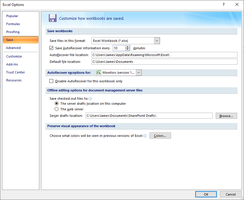
recent work was aggravating, so I decided to change the frequency with
which Excel auomatically saves a file in an AutoRecover version that will
allow you to automatically recover a document if if the program hangs
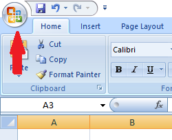
or crashes. To change that setting for Excel 2007 on a Windows system,
you can click on the Office Button at the top, left-hand corner of the
Excel window (it is to the left of the "Home" tab as shown below).
Then click on the Excel Options button and select the Save
option. The checkbox for "Save AutoRecover information every" should be
checked. You can then change the frequency from 10 minutes to a more frequent
number; I chose to have Excel automatically save a document every 5 minutes.
In the Microsoft Excel spreadsheet program, if you wish to create a dropdown
list where a user can select options from the list for a cell's value, you can
take the steps below:
Highlight the cells where you wish to have the the dropdown list appear, e.g.,
by clicking in a cell and dragging downwards through a column where a user
should select from the dropdown list.
Click on Data on the menu bar at the top of the Excel window
Click on Data Validation.
If you see 3 options under Data Validation, i.e., Data Validation,
Circle Invalid Data, and Clear Validation Circles, select Data
Validation.
You will then see a window where you can change settings. In the "Allow"
field for validation criteria, select List.
You will then be given an option to provide the items for the list in
the source field. If you have just a couple of options for the list
that won't change, you can type them separated by a comma.
Click on OK.
In cells where you have chosen to present a dropdown list to a user,
when the user clicks on the cell or tabs into it, he/she will see a
small box with a downward pointing arrowhead appear to the right of
the cell. The user can then either type a value in the field or he/she
can chose a value from the dropdown list by clicking on the small
box with the downard pointing arrowhead. If the user types a value
that isn't in the list rather than selecting from the dropdown list,
when the user hits enter or moves the cursor out of the cell, he/she
will see the message "The value you entered is not valid. A user has
restricted values that can be entered in this cell."
I needed to compare two Excel workbooks produced with Microsoft Excel for
Mac (version 16.29) on my
MacBook
Pro laptop. Unfortunately, the MAC version of Excel doesn't include a
capability to directly compare two workbooks. Since both workbooks only had one
worksheet in them, I created a new workbook and then copied the
contents of the worksheet in the first workbook to Sheet1 in the
new workbook and the contents of the worksheet in the second workbook
to Sheet2 in the new workbook. I copied the contents of the
worksheets by selecting Edit and then Select All
in a worksheet and then pasting the contents into a sheet in the
new workbook. I then created a third worksheet, Sheet3 in the new
workbook. In cell A1 in that workbook, I put the formula
=IF(Sheet1!A1 <> Sheet2!A1, "Sheet1:"&Sheet1!A1&" vs
Sheet2:"&Sheet2!A1, "")
. I clicked in that cell and then
clicked on Edit and then Copy. Since the columns
in both of the worksheets I wanted to compare extended to AE with
804 rows, I then selected all of the columns from A to AE and all
rows from 1 to 804 and then clicked on Edit and then
Paste Special with All selected. I then clicked
on OK to copy the formula throughout the new worksheet.
Excel automatically updates the references so that B2, for instance,
gets the formula =IF(Sheet1!B2 <> Sheet2!B2,
"Sheet1:"&Sheet1!B2&" vs Sheet2:"&Sheet2!B2, "").
Excel then showed the differences between Sheet1 and Sheet2 in Sheet3
where I had used a formula to compare cells in the two other sheets.
If the contents of a cell differed, Excel showed the differences.
E.g. for cell A71, I saw Sheet1:I13-0003 vs Sheet2:I97-0033, since
Sheet1 had I13-0003 in that cell whereas Sheet2 had I97-0033
. If the cells matched, the corresponding cell in Sheet3 was empty.
So, even though the Mac version of Excel doesn't include the workbook
comparison feature found in Windows versions of the program described at
How to compare two Excel files for differences, you still may be able
to compare sheets in two Excel files by copying relevant sheets into a new
sheet where you can see the differences displayed. In the exmple above, the
contents of E71 in Sheet3 showed the values for the other sheets as numeric
values, though there were dates in the corresponding cells in Sheet1 and
Sheet2.
If you have an Excel workbook containing two cells that contain
a date and time and you want to know the time difference between
them in days and hours, you can subtract one from the other and get
the elapsed time between the two timestamps in days and hours by
using a custom date and time format for the cell that will hold the
results. E.g., suppose I have a
spreadsheet with the following
timestamps
in columns A and B:
A
B
C
1
Start Time
End Time
Elapsed Time
2
1/1/18 0:01
3/1/18 15:03
3
2/6/18 15:18
2/7/18 18:07
4
3/1/18 7:55
3/1/18 13:01
The cells containing the date and time have the custom format
m/d/yy h:mm.
Click on Excel at the top, left-hand corner of the Excel window and
the select Preferences.
On the Excel Preferences window, click on View in the
Authoring section.
In the View window, click on the check box next to Developer tab,
which you will see in the In Ribbon, Show section.
You can close that window by clicking on the "x" in the red circle at the
top, left-hand corner of the window. You should then see Developer
as a selectable option to the right of Data, Review, and View on the menu
bar at the top of the Excel window.
If you click on the Developer tab, you should see options that
include Visual Basic, Macros, Record Macro, Add-ins, Excel Add-ins, Button,
Group Box, Combo Box, Label, Check Box, Scroll Bar, List Box, Option Button,
and Spinner.
If you see an error message like the one below, which was produced by Microsoft
Excel for Mac 2016 on a Mac OS X system, even though you don't have the file
open currently, then you will need to delete the lock file, which
should be in the same directory as the spreadsheet.
This file is locked for editing.
Locked by: John Doe
Filename: SGRS_2017.xlsm
You can open the file as read-only.
The lock file will have the same name as the workbook you were trying
to open, but the file name will have ~$ prepended to it. To
delete the file you will need to "escape" the meaning of the dollar sign
by putting an escape character, i.e., a backslash character, immediately
before the dollar sign. I.e., use ~\$ as shown below:
$ ls -alg **SGRS_2017.xlsm
-rw-rw-r--@ 1 ABC\Domain Users  761327 Sep 13 15:57 SGRS_2017.xlsm
-rw-rw-r--@ 1 ABC\Domain Users     171 Sep 18 22:46 ~$SGRS_2017.xlsm
$ rm ~$SGRS_2017.xlsm
rm: ~.xlsm: No such file or directory
$ rm ~\$SGRS_2017.xlsm
$
Once the lock file has been deleted, you should be able to open the
file without the warning message that it is locked for editing.
You can use the LEFT and RIGHT functions in
the Microsoft Excel
spreadsheet program along with the LEN (length) function to remove the leftmost
or rightmost character from a text
string. These functions also work in
Google Sheets,
LibreOffice Calc,
which is the spreadsheet component of the
LibreOffice software
package, and
Apache OpenOffice Calc, which is the spreadsheet program included in
Apache OpenOffice,
though in the Apache OpenOffice Calc program you need to substitute semicolons
(;) for commas (,) in the formulas. E.g.,
in Apache OpenOffice Calc you would need to use =RIGHT(A5;LEN(A5) -1)
, instead of =RIGHT(A5,LEN(A5) -1) as you would in the other
programs.
Removing the leftmost character
The syntax for the RIGHT function is RIGHT(text,[numchars]).
If you don't include numchars, i.e., you use RIGHT(text)
then the value returned is the rightmost character in the string. E.g.,
if cell A1 has 1ABC in it, then =RIGHT(A1) returns
C. But suppose, instead, you want to remove the leftmost
charaacter from a string. You can use the RIGHT function to do
so. E.g., suppose I have a column of values, e.g.:
A
B
1
1ABC
2
2DEF
3
3GHI
4
4JKL
5
5MNO
If I want to remove the number at the beginning of each text
string and put the shortened strings in column B, I could, since the
strings are all 4 characters long, use =RIGHT(A1,3) in column B1
and then copy the formula down through the other cells in column B by clicking
in cell B1 and holding down the leftmost mouse button and dragging downwards
through the other cells in column B and then hitting Ctrl-D.
But suppose the strings vary in length. I.e., suppose I have a worksheet
containing the following strings in column A: