←May→
| Sun |
Mon |
Tue |
Wed |
Thu |
Fri |
Sat |
| |
|
|
|
|
1 |
2 |
| 3 |
4 |
5 |
6 |
7 |
8 |
9 |
| 10 |
11 |
12 |
13 |
14 |
15 |
16 |
| 17 |
18 |
19 |
20 |
21 |
22 |
23 |
| 24 |
25 |
26 |
27 |
28 |
29 |
30 |
| 31 |
|
|
|
|
|
|
|
|
Thu, Oct 04, 2018 9:47 pm
Extracting images from an Excel spreadsheet
I needed to extract two diagrams from a worksheet in a
Microsoft Excel workbook. The diagrams appeared to have been put in the
worksheet as an image through a copy and paste operation. I could right-click
on an image in the sheet and choose "Copy" or "Save as Picture" and for the
latter option I could choose PNG, JPEG, PDF, GIF, or BMP for the "Save as Type"
value, but I wondered what type of file Excel was using for the embedded image.
The file was a .xlsm file, which like a .xlsx file is an
Office
Open XML (OpenXML) file format that can be "unzipped" to reveal the
constituent files within it by renaming the file to have a .zip
filename extension or copying the file to a new file with a .zip extension
- see Zipping and unzipping
Excel xlsx files. So I copied the file giving the new file a .zip extension
and then extracted the contents of that file by unzipping it. I then had a
file named "[Content_Types].xml" and the following directories in the directory
where I had extracted files from the zip file:
_rels
customXml
docProps
xl
[ More Info ]
[/os/windows/office/excel]
permanent link
Sat, Jul 28, 2018 10:45 pm
Viewing and Editing Defined Names in Excel 2013
To view or edit the
defined names in the
Microsoft Excel 2013 spreadsheet program, you can take the following steps:
-
Click on the Forumulas tab at the top of the
Excel
window.
-
From the Formulas menu, select Name Manager.
In the Name Manager window, you can see the defined names.
[ More Info ]
[/os/windows/office/excel]
permanent link
Sat, Jan 07, 2017 11:12 pm
Day of the week for dates in Excel and Calc
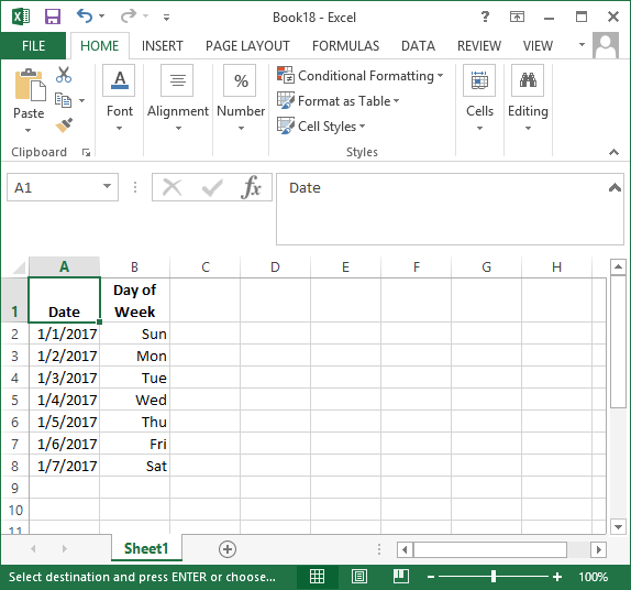
If you wish to display the day of the week, i.e, Monday, Tuesday, Wednesday,
etc., that corresponds to a particular date in
Microsoft Excel you can simply format the display of the date using
a custom format of
ddd. E.g., in Microsoft Excel 2013,
if I have dates in column A displayed in mm/dd/yyyy format, but I also
want the day of the week corresponding to those days to appear in column
B as shown below.

[ More Info ]
[/os/windows/office/excel]
permanent link
Fri, Mar 04, 2016 9:37 pm
Workday function
Sometimes you may need to determine the number of work days from one date
to another in a
Microsoft Excel,
Google Sheets, or
Apache
OpenOffice Calc spreadsheet. E.g., you may need to exclude Saturdays,
Sundays, and holidays from a calculation. All three spreadsheet programs provide
a
WORKDAY function that you can use to calculate dates based on
business work days rather than just the total number of days from a start
date. For Microsoft Excel on both Microsoft Windows and OS X and Google Sheets,
the syntax for the
WORKDAY function is as follows:
WORKDAY(start_date, num_days, [holidays])
For OpenOffice Calc, you need to separate the parameters with a semicolon
rather than a colon. I.e.:
WORKDAY(Start_date; num_days; [holidays])
If you separate the parameters with a comma in Calc, it will display
Err:508.
"Holidays" is enclosed in brackets to indicate it is an optional parameter, you
would not actually include the brackets if you specified holidays.
The arguments to the function have the following meaning:
-
Start_date - Required. A date that represents the starting date for
a calculation
-
num_days - Required. The number of nonweekend and nonholiday days before
or after the start_date. A positive value yields a future date while a negative
value yields a past date.
-
holidays - Optional. An optional list of one or more dates to exclude
from the working calendar, such as state and federal holidays and floating
holidays. The list can be either a range of cells that contain the dates
or an array constant of the serial numbers that represent the dates.
E.g., I need to determine the date when work requests that should
be completed within 5 business days after approval should be completed.
I can display the required implementation date for each request in a
worksheet by using the formula =WORKDAY(cell,5) where
cell holds the approval date. E.g., if the approval date is in cell
A2, I can set the formula for the required implemenation date to be
WORKDAY(A2,5) for Excel or Google Sheets or
WORKDAY(A2;5) for Apache OpenOffice Calc.
If there was no date in cell A2, Excel will display January 6, 1900
in the cell holding the implemenation date, e.g. 1/6/00, if
the date format is D/M/YY (day/month/2-digit year), but OpenOffice Calc
and Google Sheets will display January 5, 1900. Microsoft Excel stores
dates as sequential serial numbers so they can be used in calculations
and, by default, uses January 1, 1900 as serial number 1. If you have a
date field containing January 1, 2008 that is equivalent to 39,448, which
you would see if you put that day in a cell formatted to hold a date then
changed the format to be a number. January 1, 2016 is 42,370. January 1,
2008 is 39,448 days after January 1, 1900 and January 1, 2016 is 42,370
days after that date.
Why do Google Sheets and Apache OpenOffice Calc show January 5,
1900 as the calculated date when there is no date in the start_date
field while Microsot Excel displays January 6, 1900? Long before Microsoft
became a dominant player in the spreadsheet market,
Lotus 1-2-3
from
Lotus Development Corporation was a dominant spreadsheet in the personal
computer market. There was a bug in Lotus 1-2-3 due to the developers
assuming that the year 1900 was a leap year; it was not. When Microsoft released
Excel they had to compete with Lotus 1-2-3, the then dominant spreadsheet for
personal computers, so Microsoft needed to ensure that spreadsheets created in
Lotus 1-2-3 returned the same results in Excel, so for compatibility retained
the incorrect assumption regarding the year 1900 - see the Microsoft article
Excel incorrectly
assumes that the year 1900 is a leap year and
Excel Date Conversion (Days from 1900) regarding making an allowance for
that incorrect assumption. Google Sheets and Apache OpenOffice Calc did not
retain that incorrect assumption regarding the year 1900 and so you will
see January 5 used in certain calculations in those spreadsheets where
January 6, 1900 is used by Exel, which is why sometims you may get
differing results for date calculations between those spreadsheet
programs.
If an argument to the workday function is not a valid
date, e.g., 2/30/16 for February 30, 2016, which is not a valid date,
you will see #VALUE! displayed by the function in all three
spreadsheets. In all three spreadsheets, if days is not an integer, the
number is truncated to an integer value. E.g., if you used the formula
=WORKDAY(A2,5.7) you would get the same result as entering
WORKDAY(A2,5).
[/os/windows/office/excel]
permanent link
Tue, Jan 05, 2016 9:56 pm
Calculating an end date given the number of weeks from a start date
In spreadsheet programs such as
Microsoft Excel,
OpenOffice Calc, and
Google Sheets, you can determine an end date given a start date and
the number of weeks that some entry, such as a class, will last by using
the formula
=startdate + numweeks * 7. E.g.,
if the start date is January 11, 2016, which is stored in cell
C2
as 1/11/16 (assuming you are using the U.S.
MM/DD/YY
date
format) and the end date is to be stored in
D2
and the duration is 10 weeks, you could put the formula
=C2 +
10 * 7
in the
D2 cell. The result should be
3/21/16. If you wanted to know the date 10 weeks from today and
if today is January 5, 2016, you could use
=TODAY() + 10 *
7
. In mathematics and normally in computer operations the
order
of precedence results in multiplication and division having
precedence over addition and substraction, so ten will be multiplied by
seven and that result added to the current date to determine the last
day of the event.
[/os/windows/office/excel]
permanent link
Tue, Aug 18, 2015 9:38 pm
Counting number of cells with date before or equal to today
If you have a range of cells in an Excel worksheet that contain a date and
you wish to obtain a count of the number of those cells that have a date
that is prior to or equal to today, you could use the formula below, presuming
the relevant cells containing the date are in the range E2:E810:
COUNTIF(E2:E810,"<="&TODAY())
The ampersand concatenates today's date after the <=.
If you wanted a count for only those dates prior to today, but not including
today, you could replace the <= with <.
If you need to count cells based on multiple criteria, you can use
COUNTIFS. E.g., if for the above range of cells I want to
count the number of cells that not only have a date prior to or equal to today,
but only count the cells if there is some value in another cell in
the row, i.e., if the date in column E is prior or equal to today and there is
some value in column P in that row, i.e., column P is not blank, I can use
the formula below:
=COUNTIFS(E2:E810,"<="&TODAY(), P2:P810, "<>"&"")
E.g., I need to track when an expiration date stored in column E for an
item has passed, but I only want to count the entries when I've contacted the
user associated with the item notifying him that he needs to renew the item.
In column P in the worksheet, I store the date I contacted the user. If I
haven't yet contacted the user, the cell is empty.
I also want to now how many expiration notices I sent today, so use the
formula below for that number:
=COUNTIFS(E2:E810,"<="&TODAY(), P2:P810, "="&TODAY())
The formula checks the values in column E from E2 to E810 to determine
if the date in those cells is less than or equal to today and, if so,
whether today's date is in the corresponding cell in column P. If both
criteria are met, then the count is incremented by 1.
References:
-
Countif greater than or equal to a date
Date: February 13, 2015
MoonPoint Support
-
Excel countifs function
Date: March 14, 2014
MoonPoint Support
-
COUNTIF in Excel - count if not blank, greater than, duplicate or unique
By:
Svetlana Cheusheva
AbleBits
[/os/windows/office/excel]
permanent link
Wed, Jun 03, 2015 10:30 pm
Importing Amazon reports into Excel 2013
To import an Amazon affiliate report into Excel 2013, download the report
as a tab separated values (TSV) report, then take the following steps in
Microsoft Excel 2013 to import the data, which can also be used for any
text file containing tab delimited data:
- Click on File.
- Click on Open.
-
Under Open select the location where the downloaded file is located and
select the report.txt file you downloaded.
-
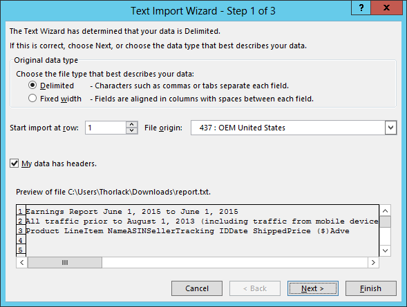
A "Text Import Wizard Step 1 of 3" window will open. You can check the check
box next to "My data has headers". You can skip the first title row, if you
wish, by changing the "Start import at row" value from the default value of 1.
Click on Next when you've made any changes needed.

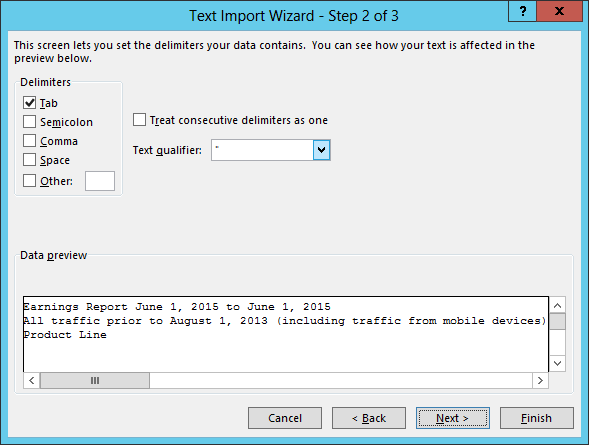
-
At step 2, leave "Tab" selected as the delimiter and click on Next.

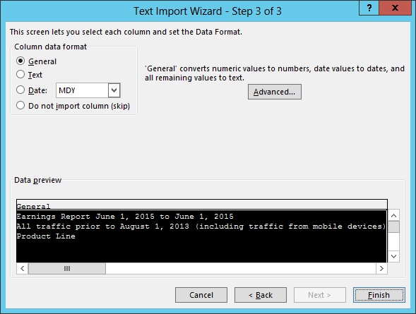
-
At step 3, you can leave "General" selected for the "Column data format" and
click on Finish.

Once the data is imported, you can click on the vertical lines between the
column headers to adjust the width of individual columns to accomodate column
titles and data. Or to have the text wrap within the current column width, you
can click on a column designator, such as "A", "B", etc., or
click on the "1" to the left of the first row to choose all columns
on that row, and then right-click and choose Format Cells,
Alignment, and then select Wrap Text under Text
Control, and then click on OK.
To save the file in an Excel spreadsheet format, select File
and Save As, select a location and name for the file, and then
change the "Save as type" value from "Text (Tab delimited) (*.txt)" to
"Excel Workbook (*.xlsx)" or other file type.
[/os/windows/office/excel]
permanent link
Wed, Apr 29, 2015 11:17 pm
Importing text data from a webpage into Excel 2013
I needed to import a whitelist consisting of a list of
fully
qualified domain names from a web page into a Microsoft Excel
spreadsheet. The web page was just a text file with one entry per line,
which made it easy to import data directly from the page in Excel 2013.
The steps to import such data from a web page are as follows:
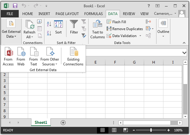
- Click on Data from the menu at the
top of the Excel window.
- Select Get External Data and From
Web.

-
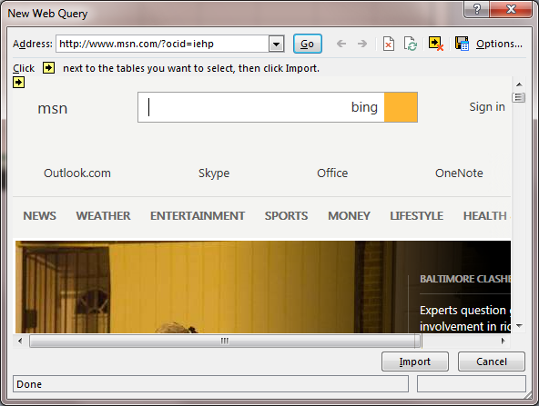
Type the URL for the webpage from which you wish to obtain the data
into the Address bar of the New Web Query window which will
have opened.

-
The contents of the webpage will be displayed and you can click on
the Import button.
-
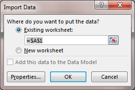
You will then be asked "Where do you want to put the data?" The default
location will be $A$1, i.e., the cell in the first column and first row.

You can change the location or leave it as is and then click on
OK to have the data inserted in the sheet in the Excel workbook
If you need to update the data from the webpage when working in the
spreadsheet later, you can select Refresh All all from the Excel
toolbar and then select Refresh.

The contents of the sheet will then be refreshed with the latest data
from the web page.
[/os/windows/office/excel]
permanent link
Thu, Feb 26, 2015 5:37 pm
Conditional formatting with "and" and "or"
I have a spreadsheet I maintain with Microsoft® Excel® 2008 for Mac
that I use to track work requests. I color code cells in the spreadsheet so
that I can easily identify requests requiring attention or that I need to
keep a closer eye on. I use Excel's conditional formatting capability to
implement the color coding. Excel only provides a maximum of 3 conditions for
conditional formatting, but you can employ formulas using the
logical "and" and "or" connectives to use multiple criteria
for an individual condition to provide additional flexibility with conditional formatting.
E.g., I have an "Expedite" column, column "O", in the spreadsheet
where I place a "Y", if the work request requires an expedited
implementation. The normal implementation time should be within 5
business days, but sometimes requests require a more immediate
implementation. I also have a status column, column "B", that
shows whether a request has been completed or is in some other state,
such as "approved", "pending", "clarification required", etc. In
any case where there is a "Y" in the Expedite column and the value
in the status column doesn't equal "Completed", I want to make the
background of the cell where the "Y" appears in the Expedite column
red, so I can easily spot ones that I need to track closely to
ensure they are completed by the given deadline for the request. I
can easily do that with conditional formatting.
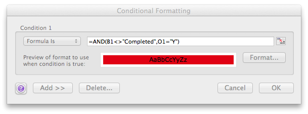
To apply that formatting, I can click on one of the cells in column "O", which
is the "Expedite" column and then click on Format and
select Conditional Formatting and set a formula for the cell.
E.g., if I've selected the first row in the spreadsheet, I can use the
formula below:
=AND(B1<>"Completed",O1="Y")
The formula specifies that if cell B1 doesn't contain the text "Completed"
and cell O1 contains "Y", then the condition is met. I can click on
the Format button and then pick the color I want to apply
to the cell background, in this case I want it colored red. Conditions that
form the logical
conjunction are separated by commas.

You can also apply
conditional formatting with an "or" condition and copy the conditional
formatting to other cells as explained there.
[/os/windows/office/excel]
permanent link
Fri, Feb 13, 2015 4:50 pm
Countif greater than or equal to a date
If you want to determine the number of entries in a spreadsheet that have
a date value that is greater than or equal to a particular date, you can
use the
COUNTIF function in Excel. E.g., if you had dates
in column G rows 4 through 959 and wished to know the number of rows
with a date that was greater than or equal to October 15, 2014, you could
use the formula below, assuming you are using the common U.S. style of date
in the form mm/dd/yyyy.
=COUNTIF(G4:G959,">=10/15/2014")
Suppose, instead, that you had a date in F970 and you wished to use
whatever date you had in that cell for the date comparision operation.
You could then use the following formula:
=COUNTIF(G4:G959,">="&F970)
The ampersand before the F970 concatenates the value in that cell to
the string >=, so that if cell F970 contains the date value
10/15/2014, COUNTIF will only count cells containing a date
greater than or equal to that date.
[/os/windows/office/excel]
permanent link

Privacy Policy
Contact


